Tuesday, July 29, 2014

GTO Poker and Multiple Equilibria Part 2

Today I'm going to continue examining GTO play in games with multiple equilibria.  I'm going to focus this post entirely on zero sum two player games and we'll take a look at various GTO strategies and how they perform against different types of fish.

If you haven't already, be sure to check out part 1 of this post where we observed that in two player zero sum games when both players play GTO strategies their EVs are the same no matter which equilibrium strategy they play but that against fish some GTO strategies performed better than others.

In the previous post we looked at a river situation with multiple GTO strategies one of which performed as well or better against all types of suboptimal play than all other GTO strategies.  Today I'm going to start by showing a very simple example of a game with multiple GTO strategies where every strategy performs better against one type suboptiaml player and worse against another type, such that there is no "best" GTO strategy.

The key take away that I want to convey is that contrary to popular belief, it is entirely possible to alter your strategy in an exploitative fashion to take advantage of your opponent while continuing to play GTO in all sorts of zero sum games including poker.

Contrived Example: AB Game


I'm going to start by introducing a totally made up game that has no bearing in reality.  As an actual game, it is quite boring, but it actually does a very good job of illustrating the general concept of how a game might have multiple GTO strategies each of which is better against a different type of fish.

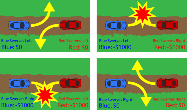
The game works as follows.  Each player privately chooses one of four options, a, A, b, or B.  They then simultaneously reveal their choice and a winner is determined.  The loser must pay the winner a dollar, if there is a tie no money is exchanged  The options are ranked as follows:  A and a both tie b and B, however A beats a and B beats b.

From examining this game it should be quite clear what the set of GTO strategies is.  In all cases, playing A is as good or better than playing a because if your opponent plays b or B you tie either way, but if he plays A you lose when you play a instead of tying.  Because the exact some logic holds for B, it cannot be GTO to ever play either a or b if a GTO player would ever play A or B which he would.

It turns out that any strategy that always plays either A or B with some frequency is GTO in this game, so always playing A is GTO, always playing B is GTO and in general playing A x% and B (1-x)% is GTO for all x in [0,1].  This is easy to verify so I won't check it here.  When two GTO players play each other they always tie so their EVs are 0.

Now lets think about performance against suboptimal play.  Suppose there are 2 fish, Fish a and Fish b.  Fish a always plays a and Fish b always plays b.  The GTO strategy that always plays A, wins every time against Fish a and breaks even against Fish b.  The GTO strategy that always plays B wins every time against Fish b and breaks even against Fish a.  Furthermore, these GTO strategies are actually maximally exploitative against the fish they exploit.

The result of this is that there is room to be exploitative and adapt your strategy to your opponent while still remaining GTO.  Imagine you are actually playing 100 rounds of this game against a random opponent from a pool of fishy opponents, some of whom play various GTO strategies, some of whom play a more often than they play b and others who do the opposite.

It would be 100% reasonable (and far more profitable than picking a specific GTO strategy and sticking to it) to have a default GTO strategy that you usually play, say always playing A, and deviating to an alternate GTO strategy as soon as you saw that your opponent played b more than me played a.

Note that in this case the behavior that we are adapting exploitatively is on the equilibrium path and when we play against a GTO opponent our strategy change will be observable to them.  We are actually switching which equilibrium strategy we are playing.  As we'll see below, there is another way to exploit opponent tendencies while remaining GTO that involves only altering our play when our opponent takes actions that are off the equilibrium path.

A Poker Example -- GTO Wiggle Room


I'm going to try and look at a somewhat real world scenario that might emerge in a HU game in a 3-bet pot on a draw heavy board.  I kept the ranges unrealistically small for simplicity and wasn't careful to precisely model accurate stack sizes because this example is designed to be illustrative of a broadly applicable concept, not to accurately address a specific situation.

Imagine we're on the river, on a draw heavy board where the river card completed the flush.  The OOP players range consists of strong over pairs, while the IP players range consists of busted sraight draws, made flush draws, and a hand full of sets and two pairs.

Specifically:

  1. The board is: 2sTs9c5h3s
  2. The IP range is: 22, 87, T9, QJ, Ks8s+, As2s-AsJs, 7s6s, 9s8s, Qs9s
  3. The OOP range is: QQ+
  4. There are 100 chips in the pot and 150 left to bet
You can view GTO play for this scenario below:


One of the first things we can note about GTO play is that the OOP player should never bet half pot when his opponent is playing GTO.  What this means is that if we run into a sub-optimal player who does bet half pot at us we have some "wiggle room" where we can adjust our strategy a bit to exploit the type of range that we think he is betting half pot with. We still remaining GTO after the exploitative adjustment so long as we don't adjust our strategy so much that a GTO player would be able to increase his profit by exploiting our adjustment by betting half pot at us with some range.

Because in this type of situation, betting from OOP is just a fundamentally weak play (similar to playing little a or litle b in the game above), there are generally going to be many different reactions to such a bet that will still be low enough EV for a best responding opponent that from his perspective, checking is still more profitable for them than betting, even if our response to the bet is unbalanced.

Specifically lets consider two potential fish types, both of whom are going to randomly lead for half pot with their entire range 10% of the time.  Fish 1 is thinking that "when he shoves here he's never bluffing" and is feeling you out with his bet and plans to fold to a shove 100%.  Fish 2 is thinking "OMG I haz overpair" and is planning to call a shove 100%.

The question I'm going to look at in part 3 is this: is there enough wiggle room that we can have two significantly different and more profitable strategies that exploit Fish 1 and Fish 2 respectively, but that are still both unexploitable enough  when our opponent leads out for 1/2 pot to be GTO?

Stay tuned... Hopefully part 3 of this post will be out in the next week or two :)

Thursday, July 17, 2014

GTO Poker and Multiple Equilibria Part 1

Today I'm goint to take a look at games with multiple equilibria (which includes poker) and discuss the implications of multiple equilibria on GTO strategies.  Because this is a large topic I'll be breaking this discussion into two separate posts.

Understanding games with multiple equilibria is important, because in practice most reasonably complex games have more than one equilibrium and in many cases some equilibria are superior to others.  Because of this, understanding the spectrum of equilibria and their properties in depth is an important part of game theory.

Coordination Games


Coordination games are the simplest examples of games with multiple equilibria.  I'll walk through a simple example that is sometimes called the "swerving game".

Imagine you are speeding along a narrow country road.  You come over a steep hill and realize another car is coming straight at you and you are both driving in the center of the road.  Furthermore, you are both going fast enough that there is no time to break.  If you both swerve to the right you will pass each other and avoid an accident.  Similarly if you both swerve to the left there will be no accident.  In both these cases your payoff is $0.  However, if you swerve to your right and the other driver swerves to his left, or if you swerve to your left and the other driver swerves to his right you will crash and both incur $1,000 of expenses.


The Swerve Game


It turns out that this game actually has three equilibria.  To see this just recall the definition of a nash equilibrium.  Suppose both players strategy is to swerve to their right.  Clearly neither player would want to deviate as that would cause a crash so the strategy pair where both players always go right is an equilibrium.  Similarly if both players always swerve to their left that is an equilibrium as well.  Both of these equilibrium outcomes give each player $0 in EV.

The third equilibrium is more subtle.  Imagine playing this game against a player who randomly goes left half the time or right half the time.  In this case no matter what strategy you employ, your EV is -$500, so all strategies are a best response to your opponents actions.  This means that both drivers swerving right 50% and left 50% is also an equilibrium, however the EV of this equilibrium is much worse for both players.  On average both players lose $500 in EV if they play this equilibrium.

Obviously in this situation everyone would be much better off if they could coordinate and agree in advance that any time they encounter such a situation they will pick one of the pure equilibrium strategies (always go right or always go left) and always play it.

In this game always going right or always going left are both "GTO" strategies in the sense that in isolation they are something a person playing optimally might do, however an equilibrium is a condition on the set of strategies that both players are using, not on a specific players strategy in isolation.  If you were in a country where people usually drive on the right, for example, such that society had coordinated on a specific equilibrium, deciding to play the strategy where you always go left would still be "GTO" technically, but in practice it would be a bad idea.

Furthermore, if you ended up in a world where somehow everyone was playing the mixed strategy equilibrium that would be terrible for everyone, even though theoretically speaking everyone would be playing GTO.  Some theorists even argue that social and cultural norms often emerge to solve coordination problems by establishing an implicit agreement on which equilibria to play.

In general, most complex games have many equilibrium and some may be better for a particular player than another at his opponents expense, or some may just be better or worse for everyone as in the swerving game.  There are a variety of ways of categorizing and classifying equilibria and trying to predict which ones are more likely to be played in practice than others (for example in the swerving game the mixed strategy equilibrium is not evolutionarily stable and thus is not something I'd expect to ever encounter in real life) but overall differentiating "good" equilibrium from bad ones and trying to predict which equilibrium outcomes will occur is a very complex problem. 

Zero Sum Games to the Rescue (sort of)


In zero sum two player games (like heads up poker situations) life is a bit simpler thanks to a key theorem.  In two player zero sum games, while their may be many different equilibrium strategies, it is the case that when both players play equilibrium strategies their EV is the same, no matter which equilibrium strategy either player chooses.  Thus if a single player is playing a GTO strategy in isolation his EV is guaranteed no matter what his opponent does.  There are no good or bad equilibrium for either player if both players stick to GTO play.

However, there still are many situations where certain GTO strategies perform better against all non-optimal opponents or against specific non-optimal opponents.  To see this, lets start by looking at a simple example of a slight variant of the [0,1] game from The Mathematics of Poker (which is a variant of a much older game solved by von Neumann and Morgenstern).  The game works as follows:

  1. There is a pot of 100 chips and both players have 100 chip stacks
  2. Both players are dealt a single card which has a number randomly chosen from between 0 and 1 (inclusive)
  3. Player 1 can bet 100% pot or check.  Player 2 can call or fold if player 1 bets, if player 1 checks then he must check back
  4. Higher numbered cards win at showdown

I walk through how to solve this game in detail in The Theory of Winning Part 2 so I will  just gloss over the solution to the game in this post.

It turns out that GTO play for the betting player is to bet the top of his range for value (all hands stronger than some value v) and the bottom of his range as a bluff (all hands worse than some value b).  The calling player than calls with the top of his range (all hands stronger than some value v).


It is relatively straight forwards to solve for the exact optimal values which are shown below.


This is a GTO solution to this game, and in this case I think it is quite clear that this is the best GTO solution, however, it turns out that while there is a unique GTO strategy for the betting player, there are infinitely many GTO strategies for the caller in this game and thus infinitely many equilibria.

To see why, just consider Player 2's decision when he holds a hand between 1/9 and 7/9 and his opponent bets.  Against a GTO opponent these hands all have exactly the same EV for both calling and folding.  Furthermore, a value bet is only more profitable than a check for Player 1 with a hand of strength x if the x beats at least half of the opponents calling range.

Suppose that rather than calling with all hands better than 5/9, the Player 2 instead calls with all hands better than 6/9 as well as hands between 4/9 and 5/9 and folds everything else.  Player 2's EV is exactly the same in this situation and for Player 1, any hand of strength less than v still looses to more than half of the callers calling range so there is no incentive for him to alter his value betting.  Furthermore, Player 2 is calling and beating bluffs with the exact some frequency so there is no reason for Player 1 to alter his betting strategy.

Thus we have another GTO strategy for Player 2, and it is easy to see that infinitely many similar strategies that shift the bottom of Player 2's calling range are all also GTO.

Now we know that against a GTO opponent both of these GTO strategies for player 2 have equal EV, but what about against a sub-optimal player 1 who value bets too wide with all hands stronger than 5/9 (instead of the GTO cutoff of 7/9) and bluffs according to GTO with hands less than 1/9.  Call him SubOptimal1.

The EVs are equal in all cases, except when SubOptimal1 has a hand between 5/9 and 6/9 and player 2 has a hand between 4/9 and 6/9.  In this case the GTO strategy where player 2 calls with hands 5/9 and better ends up calling half the time and winning half the time when he calls so his EV in this situation is one quarter of the pot, or 25 chips.

The alternate player 2 GTO strategy that calls with 4/9-5/9 and folds 5/9-6/9 ends up calling half the time and always losing a pot sized bet when he calls for an EV of -50 chips.  That's a 75 chip EV difference for player 2 between these two GTO strategies against SubOptimal1.

The probability of the situation where SubOptimal1 has a hand between 5/9 and 6/9 and player 2 has a hand between 4/9 and 6/9 occurring is 1/9 * 2/9 = 2/81 so the overall EV difference between the two strategies is 150/81.

Despite the fact that both strategies are GTO and must perform the same against an optimal opponent, against sub-optimal opponents different GTO strategies can perform quite differently.

In this case one GTO strategy is clearly much better than the other as there is no reason to ever call with a weaker hand over a stronger hand if raising is not an option.  The GTO strategy that calls with all hands better than 5/9 will have an equal or higher EV against all possible opponent strategies.  However as we'll see in part 2 of this post (coming soon) there are plenty of situations where there are two or more equilibrium strategies all of which are better at exploiting certain types of fish and worse at exploiting other types of fish.

This post continues in part 2.


Wednesday, July 2, 2014

GTO Brainteaser #6 Solution: Barreling and Bluffing

Today I'm going to go through the solution to the multistreet barreling / bluffing game that I introduced in the 6th brainteaser.  Learning how to solve this game illustrates most of the key concepts of multistreet GTO theory (these concepts also apply to single streets with multiple rounds of betting/raising), but there are a bunch of technical details around the concept of subgame perfection and backwards induction that I am going to gloss over here as they aren't super relevant.  I go through this game in more depth in one of my CardRunners videos "The Theory of Winning Part 3" which should be released sometime in the next few weeks.


The game was structured as follows:

There are 2 players on the turn, and the pot has 100 chips, effective stacks are 150 chips.  The Hero has a range that contains 50% nuts and 50% air and is out of position.  The Villain has a range that contains 100% medium strength hands that beat the Hero's air hands and lose to his nut hands.

For simplicity, assume that the river card will never improve either players hand.  You can also assume that the Hero is first to act (it turns out this doesn't actually matter).

The key question was, what is the EV of betting 50 chips on the turn and then having to option to bet 100 chips on the river with optimal ranges if our opponent calls optimally.  How does that compare to the EV of shoving the turn for 150 chips if the hero shoves an optimal range and the villain calls optimally.

In this post I am going to go through the math a bit quickly because I am mostly focused on demonstrating the technique of using backwards induction to solve these types of games.  For those interested, Keepitsimple had some great questions around clarifying some of the math in the comments which I answered in detail.

Backwards Induction


The basic way to solve these types of games is to work your way backwards.  You first want to solve the river with an arbitrary hand range and then that will tell you the EV for actions on the turn that put you into any possible river state.  I explained the concept of backwards induction here.  The basic idea is that you solve the later stages of the game (in this case the river) and determine the EV of playing that game when both players play optimally.  You then consider reaching that part of the game tree  as just immediately giving you the fixed EV payoff of optimal play.

What makes applying backwards induction directly here a bit tricky is that the distribution of nuts to air that the betting player will end up with on the river depends on the turn strategy he employs and his EV of the river game depends on his hand distribution at the start of the river.  This is similar to how the distribution of hands that you raise determines the starting distribution of hands that you have when considering a 4-bet.

What this means is that we have to solve a parameterized version of the river game that will tell us the EV of reaching the river with an arbitrary hand distribution before we can backwards induct to the turn.


Solving the River


Solving this river component of this game is quite simple.  Lets start by writing out the EV equations for the betting player when he holds air after bluffing the turn.  Call c, the frequency with which his opponent is calling a bet.

EV[bluff] = 200 * (1-c) - 100c
EV[give up] = 0

Indifference conditions require that any mixed strategy equilibrium has the same EV for bluffing and giving up.  Which implies:

200 * (1-c) - 100c = 0
c = 2/3

Similarly lets write the EV for the calling player.  Call a the probability that the betting player is bluffing when he bets.

EV[call] = 300 a + -100(1-a)
EV[fold] = 0

Again, a mixed strategy equilibrium requires these are equal which means:

a = 1/4

Clearly the betting player should always bet the nuts, and then he should bet enough air such that 1/4th of his betting range is air.  The calling player should call 2/3rds of the time.  There are two pure strategy equilibrium cases.  One occurs when the bettor has no nuts in his range, in which place he should never bluff and the calling player should always call.  The other occurs when more than 3/4ths of the bettors range is the nuts, in which case he always bets and the calling player should always fold.

Given these strategies, what is the EV of reaching the river for each player?

For the calling player he is indifferent between calling and folding when facing a bet so his EV is 0 when he is bet to as that is the EV of folding.  When his opponent checks and gives up with his air the calling player always wins the pot, so his overall EV for the river game is just the pot times how often he is checked to.  Call x the portion of the betting players range that is the nuts at the start of the river.  The actual value of x will be driven by the optimal turn strategies.  As we saw above, the betting player will always bet the nuts and will bet enough air that 1/4th of his betting range is air.  This means he will bet x + x/3 = 4x/3 of the time for x <= 3/4 and always for x > 3/4.

Thus, the calling players EV is then 200 * (1 - 4x/3) when x < 3/4 and 0 otherwise.

The betting players EV for reaching the river with a range that contains x nuts is then 200 * 4x/3 when x < 3/4, and 200 otherwise since the EVs must sum to the pot.

Back to the Turn


Using the results above we can now write out the EV equations for various actions on the turn.  Lets start with the calling player.  The EV of calling a 50 chip turn bet when our opponent is betting a range that is z% nuts is our expectation on the river minus the cost of a call:

EV[call] = 200(1 - 4z/3) - 50
EV[fold] = 0

These are equal when z = 9/16.  If the bettor always bets the nuts then he should bet his air 7/9ths on the turn because we start with 1/2 nuts, 1/2 air and (1/2) / (1/2 + 1/2 * 7/9) = 9/16 .  This means that on the river, the betting player has the nuts x = 9/16 which is less than 3/4 and puts us in our mixed equilibrium case.

For the betting player, his EV when betting with air is very simple because the EV of reaching the river with air is 0 when x < 3/4.  Call c the probability that the calling player calls.

EV[bluff] = 100 * (1-c)  - 50c
EV[give up] = 0

So again indifference requires that c = 2/3.

Our Solution


To summarize our GTO strategies, the betting player always bets the nuts on both streets.  On the turn he bets his air with probability 7/9, and on the river he bets with his air with probability 3/7 (since 9/16ths of his range is the nuts which he always bets and we want him to bet a range that is 1/4th air we need 3/7*7/16 to get 3/16 air).  The calling player calls in all situations with probability 2/3.

When both players follow these strategies the EV for the betting player is simple to calculate

EV[when we have air] = 0 by indifference
EV[when we have the nuts] = 100 * 1/3 (they fold the turn) + 150 * (2/3 * 1/3) (they call the turn and fold the river + 250 * (2/3 * 2/3) (they call the turn and the river) = 1600/9

Overall the betting players EV is thus 1/2(0) + 1/2 (1600/9) = 800/9

And since the game is 0 sum the calling players EV is 100/9

Along the way we assumed that the betting player always bets the nuts.  Were he to check the nuts it would be optimal for him to shove the river with his nuts and some % of his air.  As we'll see next, his EV with the nuts is lower in the game where he shoves, so deviating to checking the nuts is not profitable and this is an equilibrium.

What about shoving the turn


If we were to bet 150 on the turn lets write the EV equations for the betting and the calling player, again calling c the probability that the calling player calls, and a the probability that the betting player is bluffing when he bets.

EV[calling] = 250 * a - 150 * (1-a)
EV[folding] = 0

Indifference requires that a = 150/400 = 3/8

EV[betting air] = 100 (1-c) - 150c
EV[giving up] = 0 

Indifference reques that c = 100/250 = 2/5

The betting players EV when both players play these strategies is again simple:

EV[air] = indifference = 0
EV[nuts] = 100 * (3/5) + 250 (2/5) = 160

Overall EV = 1/2(0) + 1/2(80) = 80

So betting half pot twice is 800/9 - 80 = 80/9 chips higher in EV than jamming.

Where does this extra EV come from?


The extra EV comes from an effect that I call "Compounding the nuts".  The basic idea is that every time we bet an optimal polarized range our opponent has to treat the air component of that range as if it were nuts.  The air in that range is effectively converted to the nuts.  If we are on the turn and know that when we reach the river some of our range will be converted to the nuts, we can play the turn as though that portion of our range already is the nuts and thus bluff with a higher frequency.

This is a very powerful idea and its effect is that in situations like this where we have a polarized range, every additional street that we can use to bet increases our EV by letting us bluff wider and wider.

For those of you who are interested, I go over the concept of compounding the nuts in detail in my CardRunners video "The Theory of Winning Part 3" which should be released soon.